40 how to create a scatter plot in excel with labels

How to Create Scatter Plot In Excel - Career Karma Once you have inputted the data, select the desired columns, go to the Insert tab in Excel, select the XY Scatter Chart and choose the first scatter plot option. Now you should have a scatter graph shown in your Excel file. With this done, you need to add a chart title to the scatter plot. Use text as horizontal labels in Excel scatter plot Edit each data label individually, type a = character and click the cell that has the corresponding text. This process can be automated with the free XY Chart Labeler add-in. Excel 2013 and newer has the option to include "Value from cells" in the data label dialog. Format the data labels to your preferences and hide the original x axis labels.

How to Create a Quadrant Chart in Excel - Automate Excel First, let's add the horizontal quadrant line. Click the " Series X values" field and select the first two values from column X Value ( F2:F3 ). Move down to the " Series Y values " field, select the first two values from column Y Value ( G2:G3 ). Under " Series name ," type Horizontal line. When finished, click " OK .".

How to create a scatter plot in excel with labels

How to Make a Scatter Plot in Excel (Step-By-Step) | Create Scatter ... Select all the cells that contain data Click on the Insert tab Look for Charts group Under Chart group, you will find Scatter (X, Y) Chart Click the arrow to see the different types of scattering and bubble charts You can pause the pointer on the icons to see the preview in your document Click on Scatter Chart Present your data in a scatter chart or a line chart The following procedure will help you create a scatter chart with similar results. For this chart, we used the example worksheet data. You can copy this data to your worksheet, or you can use your own data. Copy the example worksheet data into a blank worksheet, or open the worksheet that contains the data you want to plot in a scatter chart. Scatter Plot Chart in Excel (Examples) | How To Create Scatter ... - EDUCBA Scatter Plot Chart is available in the Insert menu tab under the Charts section, which also has different types such as Scatter Scatter with Smooth Lines and Dotes, Scatter with Smooth Lines, Straight Line with Straight Lines under both 2D and 3D types. Where to find the Scatter Plot Chart in Excel?

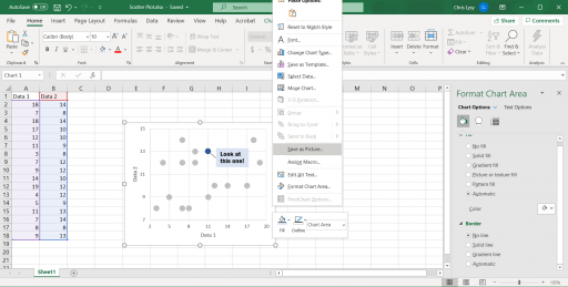
How to create a scatter plot in excel with labels. Improve your X Y Scatter Chart with custom data labels Press with right mouse button on on a chart dot and press with left mouse button on on "Add Data Labels" Press with right mouse button on on any dot again and press with left mouse button on "Format Data Labels" A new window appears to the right, deselect X and Y Value. Enable "Value from cells" Select cell range D3:D11 how to make a scatter plot in Excel - storytelling with data Highlight the two columns you want to include in your scatter plot. Then, go to the " Insert " tab of your Excel menu bar and click on the scatter plot icon in the " Recommended Charts " area of your ribbon. Select "Scatter" from the options in the "Recommended Charts" section of your ribbon. How to Make a Scatter Plot in Excel | GoSkills Create a scatter plot from the first data set by highlighting the data and using the Insert > Chart > Scatter sequence. In the above image, the Scatter with straight lines and markers was selected, but of course, any one will do. The scatter plot for your first series will be placed on the worksheet. Select the chart. How to create a scatter plot and customize data labels in Excel During Consulting Projects you will want to use a scatter plot to show potential options. Customizing data labels is not easy so today I will show you how th...

How to find, highlight and label a data point in Excel scatter plot Add the data point label. To let your users know which exactly data point is highlighted in your scatter chart, you can add a label to it. Here's how: Click on the highlighted data point to select it. Click the Chart Elements button. Select the Data Labels box and choose where to position the label. Add Custom Labels to x-y Scatter plot in Excel Step 1: Select the Data, INSERT -> Recommended Charts -> Scatter chart (3 rd chart will be scatter chart) Let the plotted scatter chart be. Step 2: Click the + symbol and add data labels by clicking it as shown below. Step 3: Now we need to add the flavor names to the label. Now right click on the label and click format data labels. How to create a Scatterplot with Dynamic Reference Lines in Excel 1. On the Developer tab, in the Controls group, click on the Insert icon and then select the Group Box (Form Control) from the Form Controls dropdown menu. 2. Next, with the mouse, draw a rectangle on the worksheet to insert the Group Box. 3. How to Add Labels to Scatterplot Points in Excel - Statology Step 3: Add Labels to Points. Next, click anywhere on the chart until a green plus (+) sign appears in the top right corner. Then click Data Labels, then click More Options…. In the Format Data Labels window that appears on the right of the screen, uncheck the box next to Y Value and check the box next to Value From Cells.

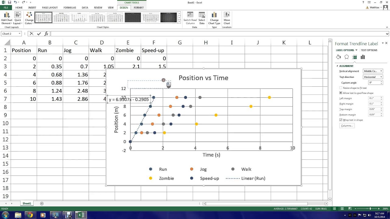
excel - How to label scatterplot points by name? - Stack Overflow select a label. When you first select, all labels for the series should get a box around them like the graph above. Select the individual label you are interested in editing. Only the label you have selected should have a box around it like the graph below. On the right hand side, as shown below, Select "TEXT OPTIONS". Microsoft Excel - Creating a Scatter Plot with trend line and axis labels A video demonstrating how to create a scatter plot, with title axis labels, and trend line on Microsoft Excel. (Also a little extra at the end on printing) Creating Scatter Plot with Marker Labels - Microsoft Community Right click any data point and click 'Add data labels and Excel will pick one of the columns you used to create the chart. Right click one of these data labels and click 'Format data labels' and in the context menu that pops up select 'Value from cells' and select the column of names and click OK. How to Make a Scatter Plot in Excel? 4 Easy Steps Option 1: Plot both variables in X vs Y scatter plot style. Use this option to check for linear relationships between variables. To implement this, just select the range of the two variables. Option 1: Select the two continuous variables. Option 2 involves plotting the variables separately in two different series.

Creating 3-D Scatter Plots - MATLAB & Simulink - MathWorks América Latina

How to display text labels in the X-axis of scatter chart in Excel? Display text labels in X-axis of scatter chart Actually, there is no way that can display text labels in the X-axis of scatter chart in Excel, but we can create a line chart and make it look like a scatter chart. 1. Select the data you use, and click Insert > Insert Line & Area Chart > Line with Markers to select a line chart. See screenshot: 2.

How To Create A Scatter Plot In Excel - slideshare

A step-by-step guide to creating a scatter plot in Excel - AilCFH Allows you to draw a scatter plot with the possibility of various semantic groupings. Some of the most common types of plots they use are replot, displot, and catplot. Creating a scatter plot in Excel: step by step Enter data and organize variables. Display the scatter chart. Add new datasets. Add titles or change axis labels. Add a trendline.

Excel 2013 - Manually adding multiple data sets to scatter plot - YouTube

How to Make a Scatter Plot in Excel to Present Your Data Consider creating a scatter plot in Excel for a great visual. Using a chart in Microsoft Excel, you can display your data visually. This makes it easy for your audience to see an attractive and ...

3d scatter plot for MS Excel

How to Make a Scatter Plot in Excel and Present Your Data Add Labels to Scatter Plot Excel Data Points You can label the data points in the X and Y chart in Microsoft Excel by following these steps: Click on any blank space of the chart and then select the Chart Elements (looks like a plus icon). Then select the Data Labels and click on the black arrow to open More Options.

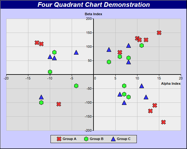
4 Quadrant Chart

X-Y Scatter Plot With Labels Excel for Mac Greetings. Excel for Mac doesn't seem to support the most basic scatter plot function - creating an X-Y plot with data labels like in the simplistic example attached. Can someone please point me towards a macro which can do this? Thank you very much in advance.

How to Create Scatter Plots in Excel - EvalCentral Blog

Scatter plot tutorial in Excel | XLSTAT Help Center Select the Visualizing data / Scatter Plot command in the XLSTAT menu. Once you have clicked on the button, the Scatter Plot dialog box appears. Groups: Satisfied. In the Options tab, activate the Frequencies and Only if >1 as we want to know if two or more points are superimposed if there is such a case. The Confidence Ellipses option can only ...

Share :