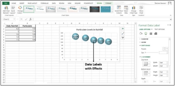
40 format data labels excel 2016

Format Data Labels in Excel- Instructions - TeachUcomp, Inc. 14.11.2019 · To format data labels in Excel, choose the set of data labels to format. To do this, click the “Format” tab within the “Chart Tools” contextual tab in the Ribbon. Then select the data labels to format from the “Chart Elements” drop-down in the “Current Selection” button group. Then click the “Format Selection” button that appears below the drop-down menu in the same … Prepare your Excel data source for a Word mail merge In your Excel data source that you'll use for a mailing list in a Word mail merge, make sure you format columns of numeric data correctly. Format a column with numbers, for example, to match a specific category such as currency. If you choose percentage as a category, be aware that the percentage format will multiply the cell value by 100 ...

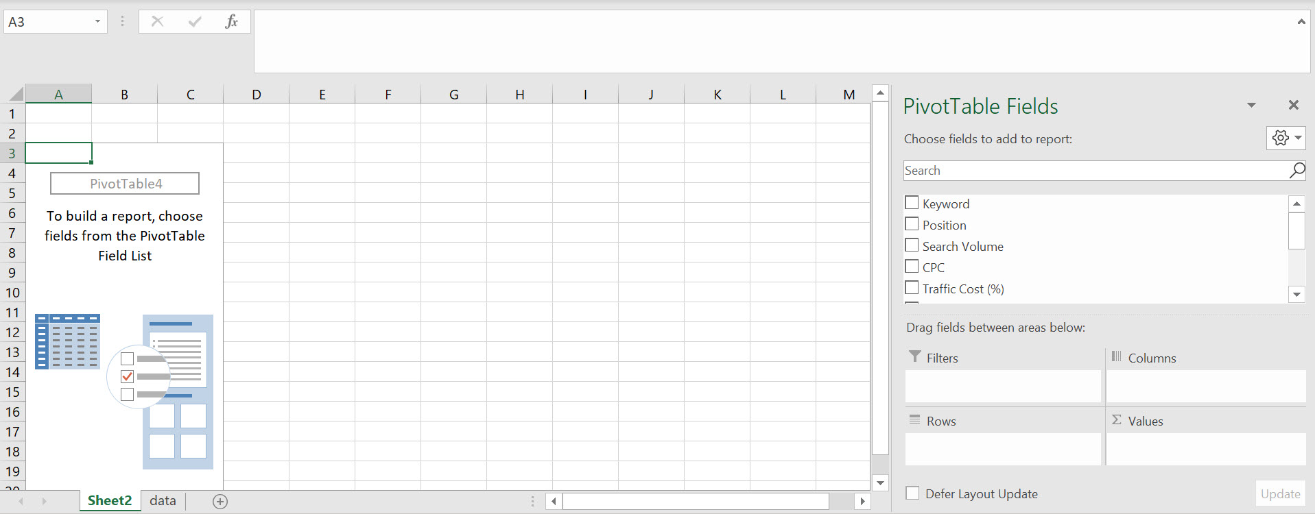
How to Format Excel Pivot Table - Contextures Excel Tips 22.06.2022 · Copy a Custom Style in Excel 2016 or Later. In Excel 2016, the custom pivot table style is not copied, if you use the above technique to copy and paste a pivot table. I found a different way to copy the custom style, and this method also works in Excel 2013. In Excel 2016, follow these steps to copy a custom style into a different workbook:

Format data labels excel 2016

How to Print Labels from Excel - Lifewire Select Mailings > Write & Insert Fields > Update Labels . Once you have the Excel spreadsheet and the Word document set up, you can merge the information and print your labels. Click Finish & Merge in the Finish group on the Mailings tab. Click Edit Individual Documents to preview how your printed labels will appear. Select All > OK . Change the format of data labels in a chart To get there, after adding your data labels, select the data label to format, and then click Chart Elements > Data Labels > More Options. To go to the appropriate area, click one of the four icons ( Fill & Line , Effects , Size & Properties ( Layout & Properties in Outlook or Word), or Label Options ) shown here. excel - Formatting chart data labels with VBA - Stack Overflow Here's the code so far: Sub FixLabels (whichchart As String) Dim cht As Chart Dim i, z As Variant Dim seriesname, seriesfmt As String Dim seriesrng As Range Set cht = Sheets ("Dashboard").ChartObjects (whichchart).Chart For i = 1 To cht.SeriesCollection.Count If cht.SeriesCollection (i).name = "#N/D" Then cht.SeriesCollection (i).DataLabels ...

Format data labels excel 2016. Excel 2016: How to Format Data and Cells - UniversalClass.com To do this, go to the Format Cells dialogue box again, and click Custom n the category column. In the Type list, select the format that you want to customize. As you can see in the snapshot above, we chose the currency format. Now go to the Type field and customize the format by entering the format you want to use. Click OK when you're finished. Edit titles or data labels in a chart - support.microsoft.com The first click selects the data labels for the whole data series, and the second click selects the individual data label. Right-click the data label, and then click Format Data Label or Format Data Labels. Click Label Options if it's not selected, and then select the Reset Label Text check box. Top of Page Excel charts: add title, customize chart axis, legend and data labels ... Click anywhere within your Excel chart, then click the Chart Elements button and check the Axis Titles box. If you want to display the title only for one axis, either horizontal or vertical, click the arrow next to Axis Titles and clear one of the boxes: Click the axis title box on the chart, and type the text. How to Customize Your Excel Pivot Chart Data Labels - dummies To remove the labels, select the None command. If you want to specify what Excel should use for the data label, choose the More Data Labels Options command from the Data Labels menu. Excel displays the Format Data Labels pane. Check the box that corresponds to the bit of pivot table or Excel table information that you want to use as the label.

How to create Custom Data Labels in Excel Charts Right click on any data label and choose the callout shape from Change Data Label Shapes option. Now adjust each data label as required to avoid overlap. Put solid fill color in the labels Finally, click on the chart (to deselect the currently selected label) and then click on a data label again (to select all data labels). 3D maps excel 2016 add data labels Re: 3D maps excel 2016 add data labels I don't think there are data labels equivalent to that in a standard chart. The bars do have a detailed tool tip but that required the map to be interactive and not a snapped picture. You could add annotation to each point. Select a stack and right click to Add annotation. Cheers Andy Move data labels - support.microsoft.com Click any data label once to select all of them, or double-click a specific data label you want to move. Right-click the selection > Chart Elements > Data Labels arrow, and select the placement option you want. Different options are available for different chart types. Format Data Labels in Excel- Instructions - TeachUcomp, Inc. Nov 14, 2019 · Alternatively, you can right-click the desired set of data labels to format within the chart. Then select the “Format Data Labels…” command from the pop-up menu that appears to format data labels in Excel. Using either method then displays the “Format Data Labels” task pane at the right side of the screen. Format Data Labels in Excel ...

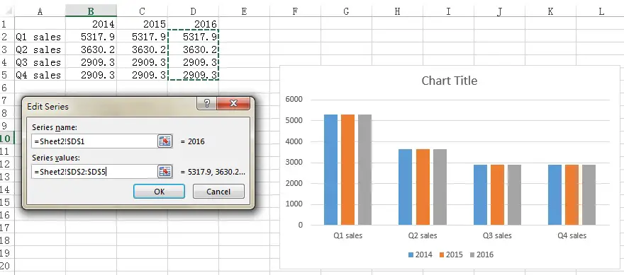
Excel Barcode Generator Add-in: Create Barcodes in Excel 2019/2016… Create 30+ barcodes into Microsoft Office Excel Spreadsheet with this Barcode Generator for Excel Add-in. No Barcode Font, Excel Macro, VBA, ActiveX control to install. Completely integrate into Microsoft Office Excel 2019, 2016, 2013, 2010 and 2007; Easy to convert text to barcode image, without any VBA, barcode font, Excel macro, formula required Change Horizontal Axis Values in Excel 2016 - AbsentData 1. Select the Chart that you have created and navigate to the Axis you want to change. 2. Right-click the axis you want to change and navigate to Select Data and the Select Data Source window will pop up, click Edit 3. The Edit Series window will open up, then you can select a series of data that you would like to change. 4. Click Ok Add or remove data labels in a chart - support.microsoft.com Click Label Options and under Label Contains, pick the options you want. Use cell values as data labels You can use cell values as data labels for your chart. Right-click the data series or data label to display more data for, and then click Format Data Labels. Click Label Options and under Label Contains, select the Values From Cells checkbox. File format reference for Word, Excel, and PowerPoint - Deploy … 30.09.2021 · The binary file format for Excel 2019, Excel 2016, Excel 2013, and Excel 2010 and Office Excel 2007. This is a fast load-and-save file format for users who need the fastest way possible to load a data file. Supports VBA projects, Excel 4.0 macro sheets, and all the new features that are used in Excel. But, this is not an XML file format and is therefore not optimal …

How to Make a Pivot Table in Excel versions: 365, 2019, 2016 and 2013 [Includes Pivot Chart]

excel - Change format of all data labels of a single series at once ... A workaround (found prior to #1): A very poor solution, but which possibly saves quite a few keystrokes/mouse clicks in many cases. Select the whole chart, and change the font size in the ribbon. It will change all text. Then recover the font size of all other text but the data labels.

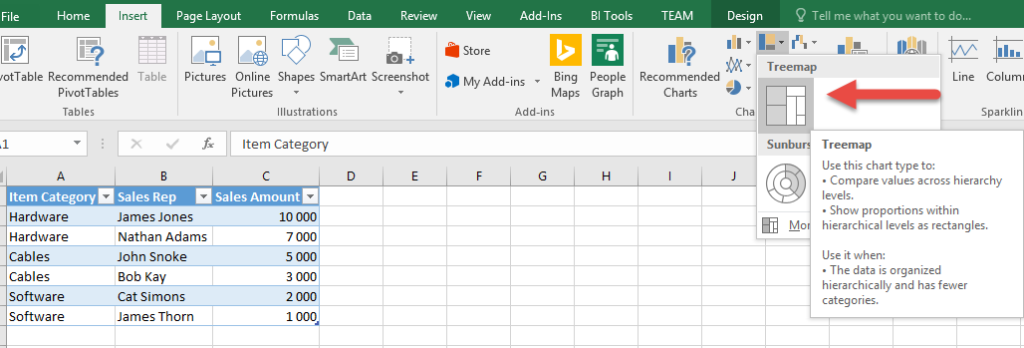
How to create a Tree Map chart in Excel 2016 | Sage Intelligence

How to add or move data labels in Excel chart? - ExtendOffice 2. Then click the Chart Elements, and check Data Labels, then you can click the arrow to choose an option about the data labels in the sub menu. See screenshot: In Excel 2010 or 2007. 1. click on the chart to show the Layout tab in the Chart Tools group. See screenshot: 2. Then click Data Labels, and select one type of data labels as you need ...

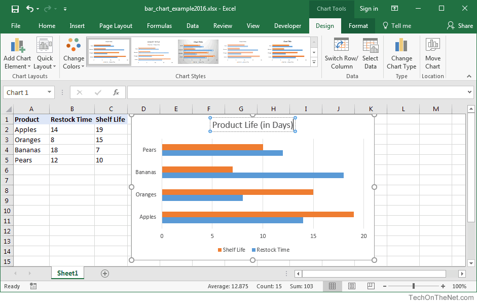
MS Office Suit Expert : MS Excel 2016: How to Create a Bar Chart

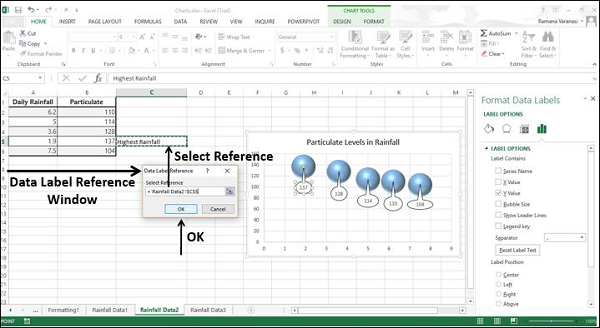
Creating a chart with dynamic labels - Microsoft Excel 2016 1. Right-click on the chart and in the popup menu, select Add Data Labels and again Add Data Labels : 2. Do one of the following: For all labels: on the Format Data Labels pane, in the Label Options, in the Label Contains group, check Value From Cells and then choose cells: For the specific label: double-click on the label value, in the popup ...

Advanced Excel - более богатые метки данных - CoderLessons.com

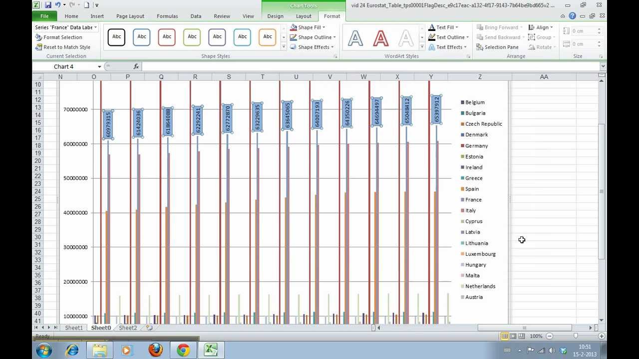
How to Change Excel Chart Data Labels to Custom Values? 05.05.2010 · Now, click on any data label. This will select “all” data labels. Now click once again. At this point excel will select only one data label. Go to Formula bar, press = and point to the cell where the data label for that chart data point is defined. Repeat the process for all other data labels, one after another. See the screencast.

Excel 3-D Pie Charts

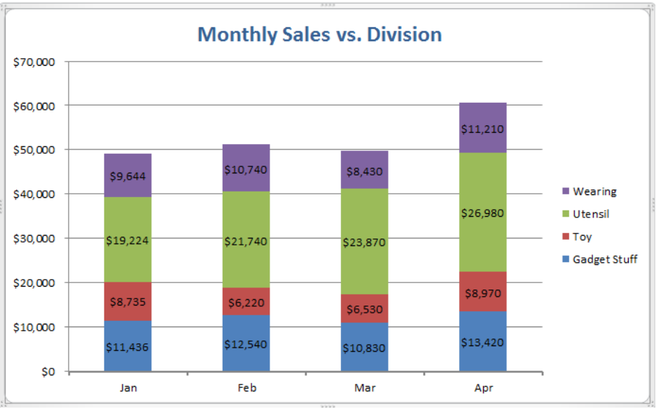
How to Add Total Data Labels to the Excel Stacked Bar Chart 03.04.2013 · Step 5: Right click your new data labels and format them so that their label position is “Above”; also make the labels bold and increase the font size . Step 6: Right click the line, select “Format Data Series”; in the Line Color menu, select “No line” Step 7: Delete the “Total” data series label within the legend. Categories Excel, Visual Design Tags charts, hacks ...

Format: Chart: Column Chart | Format | Jan's Working with Numbers

Change the format of data labels in a chart Data labels make a chart easier to understand because they show details about a data series or its individual data points. For example, in the pie chart below, without the data labels it would be difficult to tell that coffee was 38% of total sales. You can format the labels to show specific labels elements like, the percentages, series name, or category name.

32 What Is A Data Label In Excel - Labels Design Ideas 2020

How to Print Labels from Excel - Lifewire 05.04.2022 · How to Print Labels From Excel . You can print mailing labels from Excel in a matter of minutes using the mail merge feature in Word. With neat columns and rows, sorting abilities, and data entry features, Excel might be the perfect application for entering and storing information like contact lists.Once you have created a detailed list, you can use it with other …

Чарты Excel - Краткое руководство - CoderLessons.com

How to add data labels from different column in an Excel chart? This method will introduce a solution to add all data labels from a different column in an Excel chart at the same time. Please do as follows: 1. Right click the data series in the chart, and select Add Data Labels > Add Data Labels from the context menu to add data labels. 2. Right click the data series, and select Format Data Labels from the ...

Excel clustered column chart - Access-Excel.Tips

Excel 2016 for Windows - Missing data label options for scatter chart Replied on October 12, 2017. You need to use the Add Chart Element tool: either use the + at top right corner of chart, or use Chart Tools (this tab shows up only when a chart is selected) | Design | Add Chart Element. By default this will display the y-values but the Format Labels dialog lets you pick a range. best wishes.

Format Number Options for Chart Data Labels in Excel 2011 for Mac

Excel 2010: How to format ALL data point labels SIMULTANEOUSLY If you want to format all data labels for more than one series, here is one example of a VBA solution: Code: Sub x () Dim objSeries As Series With ActiveChart For Each objSeries In .SeriesCollection With objSeries.Format.Line .Transparency = 0 .Weight = 0.75 .ForeColor.RGB = 0 End With Next End With End Sub. B.

How to Add Data Labels in Excel - Excelchat | Excelchat

Create Dynamic Chart Data Labels with Slicers - Excel Campus Feb 10, 2016 · Step 3: Use the TEXT Function to Format the Labels. Typically a chart will display data labels based on the underlying source data for the chart. In Excel 2013 a new feature called “Value from Cells” was introduced. This feature allows us to specify the a range that we want to use for the labels.

Excel Custom Chart Labels • My Online Training Hub

How to Use Cell Values for Excel Chart Labels Select the chart, choose the "Chart Elements" option, click the "Data Labels" arrow, and then "More Options.". Uncheck the "Value" box and check the "Value From Cells" box. Select cells C2:C6 to use for the data label range and then click the "OK" button. The values from these cells are now used for the chart data labels.

How to Add Data Labels in an Excel Chart in Excel 2010 - YouTube

How to Add Total Data Labels to the Excel Stacked Bar Chart Apr 03, 2013 · Step 4: Right click your new line chart and select “Add Data Labels” Step 5: Right click your new data labels and format them so that their label position is “Above”; also make the labels bold and increase the font size. Step 6: Right click the line, select “Format Data Series”; in the Line Color menu, select “No line”

How to Make a Pivot Table in Excel versions: 365, 2019, 2016 and 2013 [Includes Pivot Chart]

How to hide zero data labels in chart in Excel? - ExtendOffice In the Format Data Labelsdialog, Click Numberin left pane, then selectCustom from the Categorylist box, and type #""into the Format Codetext box, and click Addbutton to add it to Typelist box. See screenshot: 3. Click Closebutton to close the dialog. Then you can see all zero data labels are hidden.

How to Add Data Labels in Excel - Excelchat | Excelchat

How to Create Mailing Labels in Excel - Excelchat Step 1 - Prepare Address list for making labels in Excel First, we will enter the headings for our list in the manner as seen below. First Name Last Name Street Address City State ZIP Code Figure 2 - Headers for mail merge Tip: Rather than create a single name column, split into small pieces for title, first name, middle name, last name.

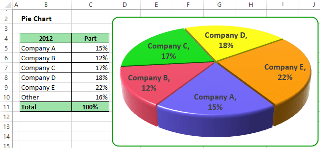
Excel 3-D Pie Charts - Microsoft Excel 2013

Excel Charts: Creating Custom Data Labels - YouTube In this video I'll show you how to add data labels to a chart in Excel and then change the range that the data labels are linked to. This video covers both W...

Share :