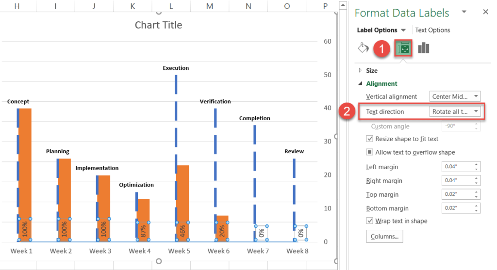
38 rotate data labels excel chart

› charts › axis-labelsHow to add Axis Labels (X & Y) in Excel & Google Sheets Edit Chart Axis Labels. Click the Axis Title; Highlight the old axis labels; Type in your new axis name; Make sure the Axis Labels are clear, concise, and easy to understand. Dynamic Axis Titles. To make your Axis titles dynamic, enter a formula for your chart title. Click on the Axis Title you want to change Reordering the Display of a Data Series (Microsoft Excel) Another way is to manually customize the chart to rearrange the data series. Follow these steps: Right-click on one of the data series that you want to move. Excel displays a Context menu. Select the Select Data option from the Context menu. Excel displays the Select Data Source dialog box. (See Figure 1.)

exceljet.net › lessons › how-to-reverse-a-chart-axisExcel tutorial: How to reverse a chart axis Let me insert a standard column chart and let's look at how Excel plots the data. When Excel plots data in a column chart, the labels run from left to right to left. In this case, the first column is Cuba, and the last is Barbados, so the columns match the order of the source data moving moving top to bottom.

Rotate data labels excel chart

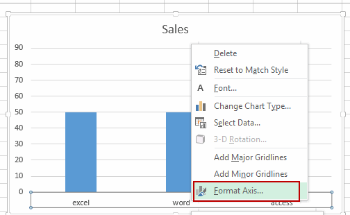
How to make shading on Excel chart and move x axis labels to the bottom ... In the Change Chart Type dialog, change the chart type for the new series to Stacked Area. Change the color from whatever Excel decides to yellow. Finally, remove the new series form the legend. See the attached version. Wi-Fi Signal Strength.xlsx 15 KB 0 Likes Reply Snoopdon replied to Hans Vogelaar Oct 24 2021 05:18 PM Format Chart Axis in Excel - Axis Options Right-click on the Vertical Axis of this chart and select the "Format Axis" option from the shortcut menu. This will open up the format axis pane at the right of your excel interface. Thereafter, Axis options and Text options are the two sub panes of the format axis pane. Formatting Chart Axis in Excel - Axis Options : Sub Panes › 509290 › how-to-use-cell-valuesHow to Use Cell Values for Excel Chart Labels Mar 12, 2020 · Select the chart, choose the “Chart Elements” option, click the “Data Labels” arrow, and then “More Options.” Uncheck the “Value” box and check the “Value From Cells” box. Select cells C2:C6 to use for the data label range and then click the “OK” button.

Rotate data labels excel chart. › charts › add-data-pointAdd Data Points to Existing Chart – Excel & Google Sheets Similar to Excel, create a line graph based on the first two columns (Months & Items Sold) Right click on graph; Select Data Range . 3. Select Add Series. 4. Click box for Select a Data Range. 5. Highlight new column and click OK. Final Graph with Single Data Point How to add secondary axis in Excel (2 easy ways) - ExcelDemy 2) Now right click on the Data Series and choose the Format Data Series option from the menu. 3) Format Data Series task pane appears on the right side of the worksheet. And we choose the Secondary Axis radio button for this data series. The keyboard shortcut to open this task pane is: CTRL + 1. › documents › excelHow to rotate axis labels in chart in Excel? - ExtendOffice Rotate axis labels in Excel 2007/2010. 1. Right click at the axis you want to rotate its labels, select Format Axis from the context menu. See screenshot: 2. In the Format Axis dialog, click Alignment tab and go to the Text Layout section to select the direction you need from the list box of Text direction. See screenshot: 3. How to Rotate Axis Labels in ggplot2? - R-bloggers How to Rotate Axis Labels in ggplot2?. Axis labels on graphs must occasionally be rotated. Let's look at how to rotate the labels on the axes in a ggplot2 plot. Let's begin by creating a basic data frame and the plot.

How to Apply a Filter to a Chart in Microsoft Excel Select the data for your chart, not the chart itself. Go to the Home tab, click the Sort & Filter drop-down arrow in the ribbon, and choose "Filter." Click the arrow at the top of the column for the chart data you want to filter. Use the Filter section of the pop-up box to filter by color, condition, or value. Advertisement Excel Waterfall Chart: How to Create One That Doesn't Suck A waterfall chart (also known as a cascade chart or a bridge chart) is a special kind of chart that illustrates how positive or negative values in a data series contribute to the total. In other words, it's an ideal way to visualize a starting value, the positive and negative changes made to that value, and the resulting end value. Pivot chart data labels rotate - Excel Help Forum For a new thread (1st post), scroll to Manage Attachments, otherwise scroll down to GO ADVANCED, click, and then scroll down to MANAGE ATTACHMENTS and click again. Now follow the instructions at the top of that screen. New Notice for experts and gurus: How to create pill charts in Excel - SpreadsheetWeb Click on Starting Space parts on the column chart. Make sure each of them is selected. Right-click on them and select No Fill as a Fill color. Apply same approach for the Ending Spaces as well. These invisible spaces gives enough gaps for hovering affect. 4. Rounding Edges This is where magic happens.

How to ☝️Make a Pie Chart in Excel (Free Template) In order to rotate a pie chart without messing up the chart title and legend, do the following: 1. Right-click on your pie chart and pick " Format Data Series " from the menu that appears. 2. Go to the " Series Option " tab. 3. How to: Display and Format Data Labels - DevExpress To specify the location of data labels on the chart, use the DataLabelBase.LabelPosition property. In this example, the DataLabelPosition.Center value is used, so data labels will be displayed centered inside columns. View Example DataLabelsActions.cs DataLabelsActions.vb DataLabel.Orientation property (Excel) | Microsoft Docs Remarks Returns or sets a Variant value that represents the text orientation. Syntax expression. Orientation expression A variable that represents a DataLabel object. Remarks The value of this property can be set to an integer value from -90 to 90 degrees or to one of the XlOrientation constants. Support and feedback How to Rotate Tick Labels in Matplotlib (With Examples) You can use the following syntax to rotate tick labels in Matplotlib plots: #rotate x-axis tick labels plt. xticks (rotation= 45) #rotate y-axis tick labels plt. yticks (rotation= 90) The following examples show how to use this syntax in practice. Example 1: Rotate X-Axis Tick Labels. The following code shows how to rotate the x-axis tick ...

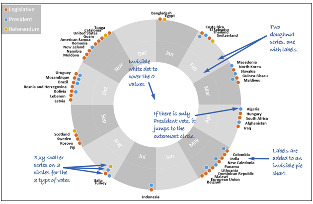
Combine pie and xy scatter charts - Advanced Excel Charting Example

Two-Level Axis Labels (Microsoft Excel) - ExcelTips (ribbon) Excel automatically recognizes that you have two rows being used for the X-axis labels, and formats the chart correctly. Since the X-axis labels appear beneath the chart data, the order of the label rows is reversed—exactly as mentioned at the first of this tip. (See Figure 1.) Figure 1. Two-level axis labels are created automatically by Excel.

How to Create a Step Chart in Excel - Automate Excel

Using Text Rotation to Create Custom Table Headers in Google Sheets Rotate up - rotate the text 90° up; Rotate down - rotate the text 90° down ... Here's an example showing a diagonal line to separate the row and column heading labels in a single cell: To achieve this, use the CHAR ... like pivot tables or charts. Generally, labels in column A need their own column heading. Alternative Way To Subdivide ...

Data Labels | FusionCharts

› documents › excelHow to group (two-level) axis labels in a chart in Excel? The Pivot Chart tool is so powerful that it can help you to create a chart with one kind of labels grouped by another kind of labels in a two-lever axis easily in Excel. You can do as follows: 1. Create a Pivot Chart with selecting the source data, and: (1) In Excel 2007 and 2010, clicking the PivotTable > PivotChart in the Tables group on the ...

Custom Data Labels with Colors and Symbols in Excel Charts - [How To] - PakAccountants.com

Make Excel charts primary and secondary axis the same scale These series may be hard to see so the easiest way to customise them is to click on the Chart, click on the Format tab, and find the series called Primary Scale. Just below this dropdown you can click on Format Selection. On the resultant options box, change the fill to No Fill and the Border to No line. You will do the same for the other new ...

How to Create a Timeline Chart in Excel - Automate Excel

How to: Display and Format Data Labels - DevExpress The example below demonstrates how to create a pie chart and adjust the display settings of its data labels. In particular, set the DataLabelBase.ShowCategoryName and DataLabelBase.ShowPercent properties to true to display the category name and percentage value in a data label at the same time.

PowerPoint: Rotate Pie Chart

How to rotate text in Google Sheets - Spreadsheet Class To make text diagonal in Google Sheets, follow these steps: Select the cell or range of cells that you want to rotate / make diagonal. Choose "Tilt up" to rotate the text diagonally upwards. Or, choose "Tilt down" to rotate the text diagonally downwards. Or, choose "Custom angle" to rotate to an angle of your preference.

How to avoid data label in excel line chart overlap with other line/label?

Matplotlib Bar Chart Labels - Python Guides Read: Matplotlib scatter marker Matplotlib bar chart labels vertical. By using the plt.bar() method we can plot the bar chart and by using the xticks(), yticks() method we can easily align the labels on the x-axis and y-axis respectively.. Here we set the rotation key to "vertical" so, we can align the bar chart labels in vertical directions.. Let's see an example of vertical aligned labels:

Label Specific Excel Chart Axis Dates • My Online Training Hub

Position labels in a paginated report chart - Microsoft Report Builder ... To change the position of point labels in a Bar chart Create a bar chart. On the design surface, right-click the chart and select Show Data Labels. Open the Properties pane. On the View tab, click Properties On the design surface, click the chart. The properties for the chart are displayed in the Properties pane.

Excel 2013 Tutorial for Beginners #65: Modifying Chart Axis, Labels, Gridlines, Etc. - YouTube

How to Rotate Text in Excel - Sheetaki First, select the cell range you want to rotate the text on. In this example, we've selected the range B1:G1, which contains our headers for months. Next, find the Orientation button. You can find this in the Alignment section under the Home tab. Click on the Orientation button to view some options you can choose to orient your text on.

How to Create a Timeline Chart in Excel - Automate Excel

Excel Dynamic Chart Linked with a Drop-down List - GeeksforGeeks Follow the below steps to implement a dynamic chart linked with a drop-down menu in Excel: Step 1: Insert the data set into an Excel sheet in the cells as shown above. Step 2: Now select any cell where you want to create the drop-down list for the courses. Step 3: Now click on the Data tab from the top of the Excel window and then click on Data ...

Excel Chart Vertical Text Labels - YouTube

How to ☝️Make a Gantt Chart in Excel - SpreadsheetDaddy 2. In the Format Cells dialog box, under " Category ," choose " Custom .". 3. In the " Type " field, enter mmm d to set a custom date format that will make it a lot easier to read the chart. Once there, here's how the dates you modified should look: Step 2. Prepare the Gantt Chart Data.

Combine pie and xy scatter charts - Advanced Excel Charting Example | Chandoo.org - Learn ...

Rotate Axis Labels of Base R Plot - GeeksforGeeks Rotate axis labels horizontally In this example, we will be rotating the axis labels of the base R plot of 10 data points to the horizontal position by the use of the plot function with the las argument with its value as 1 in the R programming language. R x = c(2, 7, 9, 1, 4, 3, 5, 6, 8, 10) y = c(10, 3, 8, 5, 6, 1, 2, 4, 9, 7) plot(x, y, las=1)

How To Rotate Text In Excel Chart - Best Picture Of Chart Anyimage.Org

How to Print Labels from Excel - Lifewire Select Mailings > Write & Insert Fields > Update Labels . Once you have the Excel spreadsheet and the Word document set up, you can merge the information and print your labels. Click Finish & Merge in the Finish group on the Mailings tab. Click Edit Individual Documents to preview how your printed labels will appear. Select All > OK .

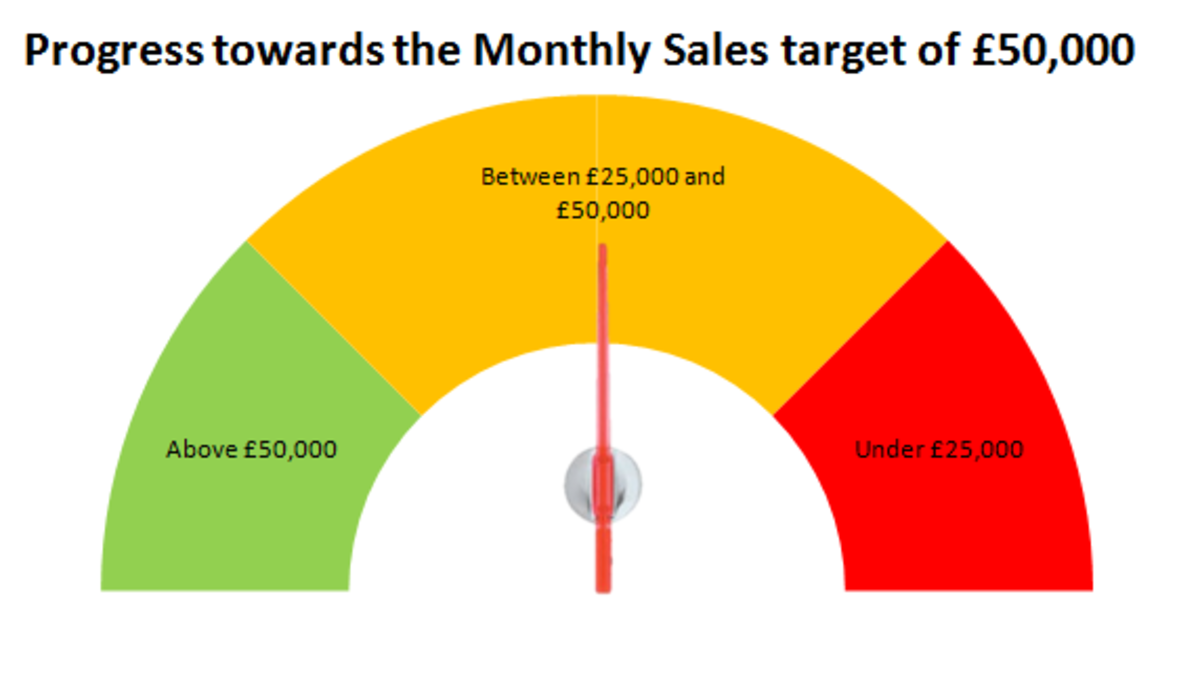
Creating a Speedometer, Dial or Gauge chart in Excel 2007 and Excel 2010 - HubPages

› 07 › 09Rotate charts in Excel - spin bar, column, pie and line charts Jul 09, 2014 · In my picture below, data labels overlap the title, which makes it look unpresentable. I am going to copy it to my PowerPoint Presentation about peoples' eating habits and want the chart to look well-ordered. To fix the issue and emphasize the most important fact, you need to know how to rotate pie chart in Excel clockwise.

34 What Is A Category Label In Excel - Labels Design Ideas 2020

Sunburst Chart in Excel - Example and Explanations In the last column , we have the size of each of the files. This column will be used to define the size of the segments. Select one of the cells in your data table. Go to the menu Insert> Hierarchical graph> Sunburst. Immediately, the sunbeams graph appears in your worksheet.

pgfplots - How to plot my data smoothly like excel does? - TeX - LaTeX Stack Exchange

How to Create and Customize a Treemap Chart in Microsoft Excel Either right-click the chart and pick "Format Chart Area" or double-click the chart to open the sidebar. On Windows, you'll see two handy buttons on the right of your chart when you select it. With these, you can add, remove, and reposition Chart Elements. And you can pick a style or color scheme with the Chart Styles button.

Adding data labels to see the value of the bars in an Excel chart

› 509290 › how-to-use-cell-valuesHow to Use Cell Values for Excel Chart Labels Mar 12, 2020 · Select the chart, choose the “Chart Elements” option, click the “Data Labels” arrow, and then “More Options.” Uncheck the “Value” box and check the “Value From Cells” box. Select cells C2:C6 to use for the data label range and then click the “OK” button.

Share :